OS Unit-3

 

2.1.1 The Process

A process is a program in execution or we can say that an instance of a running program or the entity, that can be assigned to & execute on a processor. The memory layout of a process is typically divided into multiple sections, and is shown in Figure.

These sections include:

·         Text Section—the executable code (This includes the current activity represented by the value of Program Counter and the contents of the processor's registers.)

·         Data Section—Global variables (This section contains the global and static variables.)

·         Heap Section—Memory that is dynamically allocated during program run time.

·         Stack Section—Temporary data storage when invoking functions (such as function parameters, return addresses, and local variables).

 

Figure: Layout of a process in memory.

 

A program becomes a process when an executable file is loaded into memory. Two common techniques for loading executable files are double-clicking an icon representing the executable file and entering the name of the executable file on the command line.

2.1.2 Process State

As a process executes, it changes state. The state of a process is defined in part by the current activity of that process. A process may be in one of the following states:

 

·         New State- When a program in secondary memory is started for execution, the process is said to be in a new state.

 

·         Ready State- After being loaded into the main memory and ready for execution, a process transitions from a new to a ready state. The process will now be in the ready state, waiting for the processor to execute it. Many processes may be in the ready stage in a multiprogramming environment.

 

·         Running State - After being allotted the CPU for execution, a process passes from the ready state to the run state.

 

·         Block & Wait State - If a process requires an Input/Output operation or a blocked resource during execution, it changes from run to block or the wait state.

·         The process advances to the ready state after the I/O operation is completed or the resource becomes available.

 

·         Terminate State - When a process’s execution is finished, it goes from the run state to the terminate state. The operating system deletes the process control box (or PCB) after it enters the terminate state.

 

 

Figure: Diagram of process state.

 

·        Suspend Ready State

If a process with a higher priority needs to be executed while the main memory is full, the process goes from ready to suspend ready state. Moving a lower-priority process from the ready state to the suspend ready state frees up space in the ready state for a higher-priority process. Until the main memory becomes available, the process stays in the suspend-ready state. The process is brought to its ready state when the main memory becomes accessible.

 

·        Suspend Wait State

If a process with a higher priority needs to be executed while the main memory is full, the process goes from the wait state to the suspend wait state. Moving a lower-priority process from the wait state to the suspend wait state frees up space in the ready state for a higher-priority process. The process gets moved to the suspend-ready state once the resource becomes accessible. The process is shifted to the ready state once the main memory is available.

Figure: Process States in Operation System

 

2.1.3 Process Control Block

Each process is represented in the operating system by a process control block (PCB)—also called a task control block. A PCB is shown in Figure- It contains many pieces of information associated with a specific process, including these:

 

·         Process state. The state may be new, ready, running, waiting, halted, and so on.

 

·         Program counter. The counter indicates the address of the next instruction to be executed for this process.

 

Figure: Process Control Block (PCB)

·         CPU registers. The registers vary in number and type, depending on the computer architecture. They include accumulators, index registers, stack pointers, and general-purpose registers, plus any condition-code information. Along with the program counter, this state information  must be saved when an interrupt occurs, to allow the process to be continued correctly afterward when it is rescheduled to run.

 

·         CPU-scheduling information. This information includes a process priority, pointers to scheduling queues, and any other scheduling parameters.

 

·         Memory-management information. This information may include such items as the value of the base and limit registers and the page tables, or the segment tables, depending on the memory system used by the operating system.

 

·         Accounting information. This information includes the amount of CPU and real time used, time limits, account numbers, job or process numbers, and so on.

 

·         I/O status information. This information includes the list of I/O devices allocated to the process, a list of open files, and so on.

In brief, the PCB simply serves as the repository for all the data needed to start, or restart, a process, along with some accounting data.

Process Address Space

Address space is a space in computer memory. And process Address Space means a space that is allocated in memory for a process. Every process has an address space

Address Space can be of two types

1. Physical Address Space
2. Virtual Address Space

Physical address space

The physical address is the actual location in the memory that exist physically. System access the data in the main memory, with the help of physical address. Every thing in the computer has a unique physical address. We needs to mapped it to make the address accessible. MMU is responsible for mapping.

Virtual Address Space

Virtual Address Space is an address space that is created outside the main memory inside the virtual memory, and it is created in the hard disk.

When our main memory is less and we want to get more benefit from this less memory, then we create virtual memory.

Logical Address is the address is always generated by CPU while running a program. The logical address is also called virtual address. Virtual address does not exist physically, so we can say that physical address is the logical address.

How to access the physical memory location by CPU?

Logical Address is used as a reference to access the physical memory location by CPU. The Memory-Management Unit uses the address-binding methods for mapping the logical address to its corresponding physical address.

PARAMENTER	LOGICAL ADDRESS	PHYSICAL ADDRESS
Basic	ADDRESS generated by CPU is called LOGICAL ADDRESS.	PHYSICAL ADDRESS  is the actual location in a memory unit.
Generation	generated by the CPU	Computed by MMU
Access	logical address can be used to access the physical address by the user.	The user can’t directly access physical address but it is possible indirectly.
Visibility	logical address of a program is visible to the user.	physical address of program is not visible to the user.
Address Space	set of all logical addresses generated by CPU are called logical addresses.	Addresses mapped to the corresponding logical addresses.

virtual memory

Virtual memory is memory outside the main memory and inside the hard disk

Virtual memory acts as the main memory but it is actually not the main memory

When a process is loads in OS, its address space is created.

Threads and their management

A thread is a flow of execution through the process code, with its own program counter that keeps track of which instruction to execute next, system registers which hold its current working variables, and a stack which contains the execution history.

A thread shares with its peer threads few information like code segment, data segment and open files. When one thread alters a code segment memory item, all other threads see that.

A thread is also called a lightweight process. Threads provide a way to improve application performance through parallelism. Threads represent a software approach to improving performance of operating system by reducing the overhead thread is equivalent to a classical process.

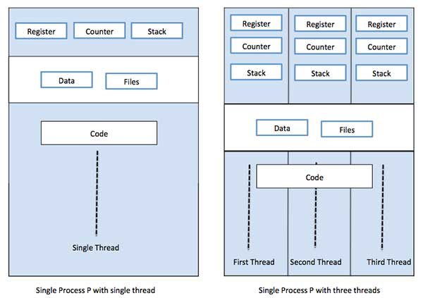
Each thread belongs to exactly one process and no thread can exist outside a process. Each thread represents a separate flow of control. Threads have been successfully used in implementing network servers and web server. They also provide a suitable foundation for parallel execution of applications on shared memory multiprocessors. The following figure shows the working of a single-threaded and a multithreaded process.

Difference between Process and Thread

S.N.	Process	Thread
1	Process is heavy weight or resource intensive.	Thread is light weight, taking lesser resources than a process.
2	Process switching needs interaction with operating system.	Thread switching does not need to interact with operating system.
3	In multiple processing environments, each process executes the same code but has its own memory and file resources.	All threads can share same set of open files, child processes.
4	If one process is blocked, then no other process can execute until the first process is unblocked.	While one thread is blocked and waiting, a second thread in the same task can run.
5	Multiple processes without using threads use more resources.	Multiple threaded processes use fewer resources.
6	In multiple processes each process operates independently of the others.	One thread can read, write or change another thread's data.

Advantages of Thread

• Threads minimize the context switching time.
• Use of threads provides concurrency within a process.
• Efficient communication.
• It is more economical to create and context switch threads.
• Threads allow utilization of multiprocessor architectures to a greater scale and efficiency.

Types of Thread

Threads are implemented in following two ways −

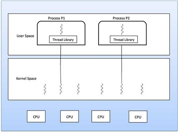
• User Level Threads − User managed threads.

• Kernel Level Threads − Operating System managed threads acting on kernel, an operating system core.

User Level Threads

In this case, the thread management kernel is not aware of the existence of threads. The thread library contains code for creating and destroying threads, for passing message and data between threads, for scheduling thread execution and for saving and restoring thread contexts. The application starts with a single thread.

Advantages

• Thread switching does not require Kernel mode privileges.
• User level thread can run on any operating system.
• Scheduling can be application specific in the user level thread.
• User level threads are fast to create and manage.

Disadvantages

• In a typical operating system, most system calls are blocking.
• Multithreaded application cannot take advantage of multiprocessing.

Kernel Level Threads

In this case, thread management is done by the Kernel. There is no thread management code in the application area. Kernel threads are supported directly by the operating system. Any application can be programmed to be multithreaded. All of the threads within an application are supported within a single process.

The Kernel maintains context information for the process as a whole and for individuals threads within the process. Scheduling by the Kernel is done on a thread basis. The Kernel performs thread creation, scheduling and management in Kernel space. Kernel threads are generally slower to create and manage than the user threads.

Advantages

• Kernel can simultaneously schedule multiple threads from the same process on multiple processes.
• If one thread in a process is blocked, the Kernel can schedule another thread of the same process.
• Kernel routines themselves can be multithreaded.

Disadvantages

• Kernel threads are generally slower to create and manage than the user threads.
• Transfer of control from one thread to another within the same process requires a mode switch to the Kernel.

Multithreading Models

Some operating system provide a combined user level thread and Kernel level thread facility. Solaris is a good example of this combined approach. In a combined system, multiple threads within the same application can run in parallel on multiple processors and a blocking system call need not block the entire process. Multithreading models are three types

• Many to many relationship.
• Many to one relationship.
• One to one relationship.

Many to Many Model

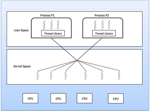
The many-to-many model multiplexes any number of user threads onto an equal or smaller number of kernel threads.

The following diagram shows the many-to-many threading model where 6 user level threads are multiplexing with 6 kernel level threads. In this model, developers can create as many user threads as necessary and the corresponding Kernel threads can run in parallel on a multiprocessor machine. This model provides the best accuracy on concurrency and when a thread performs a blocking system call, the kernel can schedule another thread for execution.

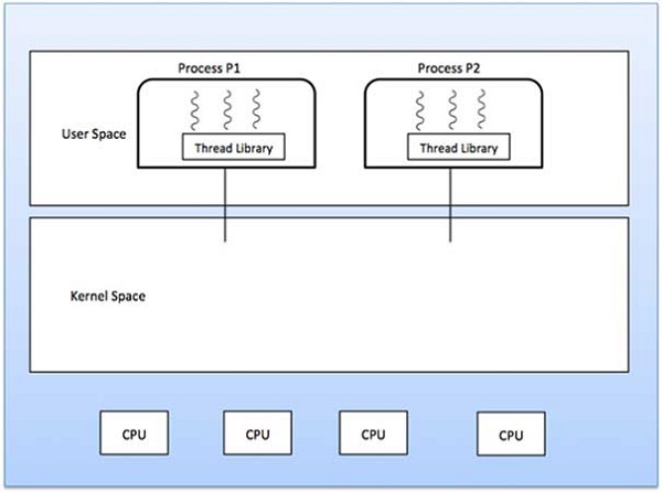
Many to One Model

Many-to-one model maps many user level threads to one Kernel-level thread. Thread management is done in user space by the thread library. When thread makes a blocking system call, the entire process will be blocked. Only one thread can access the Kernel at a time, so multiple threads are unable to run in parallel on multiprocessors.

If the user-level thread libraries are implemented in the operating system in such a way that the system does not support them, then the Kernel threads use the many-to-one relationship modes.

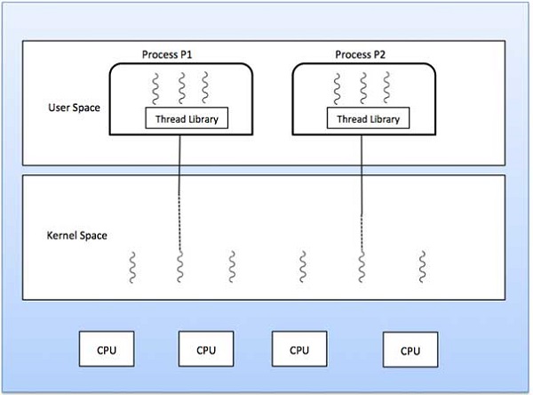
One to One Model

There is one-to-one relationship of user-level thread to the kernel-level thread. This model provides more concurrency than the many-to-one model. It also allows another thread to run when a thread makes a blocking system call. It supports multiple threads to execute in parallel on microprocessors.

Disadvantage of this model is that creating user thread requires the corresponding Kernel thread. OS/2, windows NT and windows 2000 use one to one relationship model.

Difference between User-Level & Kernel-Level Thread

S.N.	User-Level Threads	Kernel-Level Thread
1	User-level threads are faster to create and manage.	Kernel-level threads are slower to create and manage.
2	Implementation is by a thread library at the user level.	Operating system supports creation of Kernel threads.
3	User-level thread is generic and can run on any operating system.	Kernel-level thread is specific to the operating system.
4	Multi-threaded applications cannot take advantage of multiprocessing.	Kernel routines themselves can be multithreaded.

CPU Scheduling Criteria

CPU scheduling is a process that allows one process to use the CPU while the execution of another process is on hold(in waiting state) due to unavailability of any resource like I/O etc, thereby making full use of CPU. The aim of CPU scheduling is to make the system efficient, fast, and fair.

Whenever the CPU becomes idle, the operating system must select one of the processes in the ready queue to be executed. The selection process is carried out by the short-term scheduler (or CPU scheduler). The scheduler selects from among the processes in memory that are ready to execute and allocates the CPU to one of them.

Different CPU scheduling algorithms have different properties and the choice of a particular algorithm depends on the various factors. Many criteria have been suggested for comparing CPU scheduling algorithms. 

The criteria include the following: 

1. CPU utilisation – 
   The main objective of any CPU scheduling algorithm is to keep the CPU as busy as possible. Theoretically, CPU utilisation can range from 0 to 100 but in a real-time system, it varies from 40 to 90 percent depending on the load upon the system. 
    
2. Throughput – 
   A measure of the work done by CPU is the number of processes being executed and completed per unit time. This is called throughput. The throughput may vary depending upon the length or duration of processes. 
    
3. Turnaround time – 
   For a particular process, an important criteria is how long it takes to execute that process. The time elapsed from the time of submission of a process to the time of completion is known as the turnaround time. Turn-around time is the sum of times spent waiting to get into memory, waiting in ready queue, executing in CPU, and waiting for I/O. 
    
4. Waiting time – 
   A scheduling algorithm does not affect the time required to complete the process once it starts execution. It only affects the waiting time of a process i.e. time spent by a process waiting in the ready queue. 
    
5. Response time – 
   In an interactive system, turn-around time is not the best criteria. A process may produce some output fairly early and continue computing new results while previous results are being output to the user. Thus another criteria is the time taken from submission of the process of request until the first response is produced. This measure is called response time. 

FCFS Scheduling

In FCFS Scheduling,

• The process which arrives first in the ready queue is firstly assigned the CPU.
• In case of a tie, process with smaller process id is executed first.
• It is always non-preemptive in nature. 

Advantages- 

• It is simple and easy to understand.
• It can be easily implemented using queue data structure.
• It does not lead to starvation.

 Disadvantages- 

• It does not consider the priority or burst time of the processes.
• It suffers from convoy effect. 

Convoy Effect

In convoy effect, Consider processes with higher burst time arrived before the processes with smaller burst time. Then, smaller processes have to wait for a long time for longer processes to release the CPU.

 PRACTICE PROBLEMS BASED ON FCFS SCHEDULING-

 Problem-01:

 Consider the set of 5 processes whose arrival time and burst time are given below-

 

Process Id	Arrival time	Burst time
P1	3	4
P2	5	3
P3	0	2
P4	5	1
P5	4	3

 

If the CPU scheduling policy is FCFS, calculate the average waiting time and average turn around time. 

Solution-

 

Gantt Chart-

 

 

Here, black box represents the idle time of CPU.

Now, we know-

• Turn Around time = Exit time – Arrival time
• Waiting time = Turn Around time – Burst time 

Process Id	Exit time	Turn Around time	Waiting time
P1	7	7 – 3 = 4	4 – 4 = 0
P2	13	13 – 5 = 8	8 – 3 = 5
P3	2	2 – 0 = 2	2 – 2 = 0
P4	14	14 – 5 = 9	9 – 1 = 8
P5	10	10 – 4 = 6	6 – 3 = 3

 

Now,

• Average Turn Around time = (4 + 8 + 2 + 9 + 6) / 5 = 29 / 5 = 5.8 unit
• Average waiting time = (0 + 5 + 0 + 8 + 3) / 5 = 16 / 5 = 3.2 unit

 

Problem-02:

 

Consider the set of 3 processes whose arrival time and burst time are given below-

 

Process Id	Arrival time	Burst time
P1	0	2
P2	3	1
P3	5	6

 

If the CPU scheduling policy is FCFS, calculate the average waiting time and average turn around time. 

Solution-

 

Gantt Chart-

 

 

Here, black box represents the idle time of CPU.

 

Now, we know-

• Turn Around time = Exit time – Arrival time
• Waiting time = Turn Around time – Burst time

 

Process Id	Exit time	Turn Around time	Waiting time
P1	2	2 – 0 = 2	2 – 2 = 0
P2	4	4 – 3 = 1	1 – 1 = 0
P3	11	11- 5 = 6	6 – 6 = 0

 

Now,

• Average Turn Around time = (2 + 1 + 6) / 3 = 9 / 3 = 3 unit
• Average waiting time = (0 + 0 + 0) / 3 = 0 / 3 = 0 unit

 

Problem-03: 

Consider the set of 6 processes whose arrival time and burst time are given below-

 

Process Id	Arrival time	Burst time
P1	0	3
P2	1	2
P3	2	1
P4	3	4
P5	4	5
P6	5	2

 

If the CPU scheduling policy is FCFS and there is 1 unit of overhead in scheduling the processes, find the efficiency of the algorithm. 

Solution- 

Gantt Chart- 

 Here, δ denotes the context switching overhead. 

Now,

• Useless time / Wasted time = 6 x δ = 6 x 1 = 6 unit
• Total time = 23 unit
• Useful time = 23 unit – 6 unit = 17 unit 

Efficiency (η)

= Useful time / Total Total

= 17 unit / 23 unit

= 0.7391

SJF Scheduling | SRTF | CPU Scheduling

 In SJF Scheduling,

• Out of all the available processes, CPU is assigned to the process having smallest burst time.
• In case of a tie, it is broken by FCFS Scheduling. 

 

• SJF Scheduling can be used in both preemptive and non-preemptive mode.
• Preemptive mode of Shortest Job First is called as Shortest Remaining Time First (SRTF).

 

Advantages-

 

• SRTF is optimal and guarantees the minimum average waiting time.
• It provides a standard for other algorithms since no other algorithm performs better than it.

 

Disadvantages-

 

• It can not be implemented practically since burst time of the processes can not be known in advance.
• It leads to starvation for processes with larger burst time.
• Priorities can not be set for the processes.
• Processes with larger burst time have poor response time.

 

PRACTICE PROBLEMS BASED ON SJF SCHEDULING-

 

Problem-01:

 

Consider the set of 5 processes whose arrival time and burst time are given below-

 

Process Id	Arrival time	Burst time
P1	3	1
P2	1	4
P3	4	2
P4	0	6
P5	2	3

 

If the CPU scheduling policy is SJF non-preemptive, calculate the average waiting time and average turn around time. 

Solution-

 

Gantt Chart-

 

 Now, we know-

• Turn Around time = Exit time – Arrival time
• Waiting time = Turn Around time – Burst time 

Process Id	Exit time	Turn Around time	Waiting time
P1	7	7 – 3 = 4	4 – 1 = 3
P2	16	16 – 1 = 15	15 – 4 = 11
P3	9	9 – 4 = 5	5 – 2 = 3
P4	6	6 – 0 = 6	6 – 6 = 0
P5	12	12 – 2 = 10	10 – 3 = 7

 

Now,

• Average Turn Around time = (4 + 15 + 5 + 6 + 10) / 5 = 40 / 5 = 8 unit
• Average waiting time = (3 + 11 + 3 + 0 + 7) / 5 = 24 / 5 = 4.8 unit

 

Problem-02:

 

Consider the set of 5 processes whose arrival time and burst time are given below-

 

Process Id	Arrival time	Burst time
P1	3	1
P2	1	4
P3	4	2
P4	0	6
P5	2	3

 

If the CPU scheduling policy is SJF preemptive, calculate the average waiting time and average turn around time.

 

Solution-

 

Gantt Chart-

 

 

Now, we know-

• Turn Around time = Exit time – Arrival time
• Waiting time = Turn Around time – Burst time

 

Process Id	Exit time	Turn Around time	Waiting time
P1	4	4 – 3 = 1	1 – 1 = 0
P2	6	6 – 1 = 5	5 – 4 = 1
P3	8	8 – 4 = 4	4 – 2 = 2
P4	16	16 – 0 = 16	16 – 6 = 10
P5	11	11 – 2 = 9	9 – 3 = 6

 

Now,

• Average Turn Around time = (1 + 5 + 4 + 16 + 9) / 5 = 35 / 5 = 7 unit
• Average waiting time = (0 + 1 + 2 + 10 + 6) / 5 = 19 / 5 = 3.8 unit

 

Problem-03:

 

Consider the set of 6 processes whose arrival time and burst time are given below-

 

Process Id	Arrival time	Burst time
P1	0	7
P2	1	5
P3	2	3
P4	3	1
P5	4	2
P6	5	1

 

If the CPU scheduling policy is shortest remaining time first, calculate the average waiting time and average turn around time.

 

Solution-

 

Gantt Chart-

 

 

Now, we know-

• Turn Around time = Exit time – Arrival time
• Waiting time = Turn Around time – Burst time

 

Process Id	Exit time	Turn Around time	Waiting time
P1	19	19 – 0 = 19	19 – 7 = 12
P2	13	13 – 1 = 12	12 – 5 = 7
P3	6	6 – 2 = 4	4 – 3 = 1
P4	4	4 – 3 = 1	1 – 1 = 0
P5	9	9 – 4 = 5	5 – 2 = 3
P6	7	7 – 5 = 2	2 – 1 = 1

 

Now,

• Average Turn Around time = (19 + 12 + 4 + 1 + 5 + 2) / 6 = 43 / 6 = 7.17 unit
• Average waiting time = (12 + 7 + 1 + 0 + 3 + 1) / 6 = 24 / 6 = 4 unit

 

Problem-04:

 

Consider the set of 3 processes whose arrival time and burst time are given below-

 

Process Id	Arrival time	Burst time
P1	0	9
P2	1	4
P3	2	9

 

If the CPU scheduling policy is SRTF, calculate the average waiting time and average turn around time.

 

Solution-

 

Gantt Chart-

 

 

Now, we know-

• Turn Around time = Exit time – Arrival time
• Waiting time = Turn Around time – Burst time

 

Process Id	Exit time	Turn Around time	Waiting time
P1	13	13 – 0 = 13	13 – 9 = 4
P2	5	5 – 1 = 4	4 – 4 = 0
P3	22	22- 2 = 20	20 – 9 = 11

 

Now,

• Average Turn Around time = (13 + 4 + 20) / 3 = 37 / 3 = 12.33 unit
• Average waiting time = (4 + 0 + 11) / 3 = 15 / 3 = 5 unit

 

Problem-05:

 

Consider the set of 4 processes whose arrival time and burst time are given below-

 

Process Id	Arrival time	Burst time
P1	0	20
P2	15	25
P3	30	10
P4	45	15

 

If the CPU scheduling policy is SRTF, calculate the waiting time of process P2.

 

Solution-

 

Gantt Chart-

 

 

Now, we know-

• Turn Around time = Exit time – Arrival time
• Waiting time = Turn Around time – Burst time

Thus,

• Turn Around Time of process P2 = 55 – 15 = 40 unit
• Waiting time of process P2 = 40 – 25 = 15 unit

 

Implementation of Algorithm-

 

• Practically, the algorithm can not be implemented but theoretically it can be implemented.
• Among all the available processes, the process with smallest burst time has to be selected.
• Min heap is a suitable data structure where root element contains the process with least burst time.
• In min heap, each process will be added and deleted exactly once.
• Adding an element takes log(n) time and deleting an element takes log(n) time.
• Thus, for n processes, time complexity = n x 2log(n) = nlog(n)

 

To gain better understanding about SJF Scheduling,

Priority Scheduling

In Priority Scheduling,

• Out of all the available processes, CPU is assigned to the process having the highest priority.
• In case of a tie, it is broken by FCFS Scheduling. 

 

• Priority Scheduling can be used in both preemptive and non-preemptive mode.

 

Advantages- 

• It considers the priority of the processes and allows the important processes to run first.
• Priority scheduling in preemptive mode is best suited for real time operating system.

 

Disadvantages- 

• Processes with lesser priority may starve for CPU.
• There is no idea of response time and waiting time.

 

Important Notes-

 

Note-01:

 

• The waiting time for the process having the highest priority will always be zero in preemptive mode.
• The waiting time for the process having the highest priority may not be zero in non-preemptive mode.

 

Note-02:

 

Priority scheduling in preemptive and non-preemptive mode behaves exactly same under following conditions-

• The arrival time of all the processes is same
• All the processes become available

 

PRACTICE PROBLEMS BASED ON PRIORITY SCHEDULING-

 

Problem-01:

 

Consider the set of 5 processes whose arrival time and burst time are given below-

 

Process Id	Arrival time	Burst time	Priority
P1	0	4	2
P2	1	3	3
P3	2	1	4
P4	3	5	5
P5	4	2	5

 

If the CPU scheduling policy is priority non-preemptive, calculate the average waiting time and average turn around time. (Higher number represents higher priority)

 

Solution-

 

Gantt Chart-

 

 

Now, we know-

• Turn Around time = Exit time – Arrival time
• Waiting time = Turn Around time – Burst time

  

Process Id	Exit time	Turn Around time	Waiting time
P1	4	4 – 0 = 4	4 – 4 = 0
P2	15	15 – 1 = 14	14 – 3 = 11
P3	12	12 – 2 = 10	10 – 1 = 9
P4	9	9 – 3 = 6	6 – 5 = 1
P5	11	11 – 4 = 7	7 – 2 = 5

 

Now,

• Average Turn Around time = (4 + 14 + 10 + 6 + 7) / 5 = 41 / 5 = 8.2 unit
• Average waiting time = (0 + 11 + 9 + 1 + 5) / 5 = 26 / 5 = 5.2 unit

 

Problem-02:

 

Consider the set of 5 processes whose arrival time and burst time are given below-

 

Process Id	Arrival time	Burst time	Priority
P1	0	4	2
P2	1	3	3
P3	2	1	4
P4	3	5	5
P5	4	2	5

 

If the CPU scheduling policy is priority preemptive, calculate the average waiting time and average turn around time. (Higher number represents higher priority) 

Solution-

 

Gantt Chart-

 

 

Now, we know-

• Turn Around time = Exit time – Arrival time
• Waiting time = Turn Around time – Burst time

 

Process Id	Exit time	Turn Around time	Waiting time
P1	15	15 – 0 = 15	15 – 4 = 11
P2	12	12 – 1 = 11	11 – 3 = 8
P3	3	3 – 2 = 1	1 – 1 = 0
P4	8	8 – 3 = 5	5 – 5 = 0
P5	10	10 – 4 = 6	6 – 2 = 4

 

Now,

• Average Turn Around time = (15 + 11 + 1 + 5 + 6) / 5 = 38 / 5 = 7.6 unit
• Average waiting time = (11 + 8 + 0 + 0 + 4) / 5 = 23 / 5 = 4.6 unit

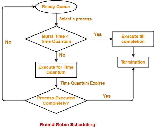
Round Robin Scheduling

In Round Robin Scheduling,

• CPU is assigned to the process on the basis of FCFS for a fixed amount of time.
• This fixed amount of time is called as time quantum or time slice.
• After the time quantum expires, the running process is preempted and sent to the ready queue.
• Then, the processor is assigned to the next arrived process.
• It is always preemptive in nature.

 

Round Robin Scheduling is FCFS Scheduling with preemptive mode.

 

 Advantages- 

• It gives the best performance in terms of average response time.
• It is best suited for time sharing system, client server architecture and interactive system.

 

Disadvantages- 

• It leads to starvation for processes with larger burst time as they have to repeat the cycle many times.
• Its performance heavily depends on time quantum.
• Priorities can not be set for the processes.

 

Important Notes- 

Note-01:

 

With decreasing value of time quantum,

• Number of context switch increases
• Response time decreases
• Chances of starvation decreases

 

Thus, smaller value of time quantum is better in terms of response time.

 

Note-02:

 

With increasing value of time quantum,

• Number of context switch decreases
• Response time increases
• Chances of starvation increases

 

Thus, higher value of time quantum is better in terms of number of context switch.

 

Note-03:

 

• With increasing value of time quantum, Round Robin Scheduling tends to become FCFS Scheduling.
• When time quantum tends to infinity, Round Robin Scheduling becomes FCFS Scheduling.

 

Note-04:

 

• The performance of Round Robin scheduling heavily depends on the value of time quantum.
• The value of time quantum should be such that it is neither too big nor too small.

 

PRACTICE PROBLEMS BASED ON ROUND ROBIN SCHEDULING-

 

Problem-01:

 

Consider the set of 5 processes whose arrival time and burst time are given below-

 

Process Id	Arrival time	Burst time
P1	0	5
P2	1	3
P3	2	1
P4	3	2
P5	4	3

 

If the CPU scheduling policy is Round Robin with time quantum = 2 unit, calculate the average waiting time and average turn around time.

 

Solution-

 

Gantt Chart-

 

Ready Queue-

P5, P1, P2, P5, P4, P1, P3, P2, P1

 

 Now, we know-

• Turn Around time = Exit time – Arrival time
• Waiting time = Turn Around time – Burst time 

Process Id	Exit time	Turn Around time	Waiting time
P1	13	13 – 0 = 13	13 – 5 = 8
P2	12	12 – 1 = 11	11 – 3 = 8
P3	5	5 – 2 = 3	3 – 1 = 2
P4	9	9 – 3 = 6	6 – 2 = 4
P5	14	14 – 4 = 10	10 – 3 = 7

 

Now,

• Average Turn Around time = (13 + 11 + 3 + 6 + 10) / 5 = 43 / 5 = 8.6 unit
• Average waiting time = (8 + 8 + 2 + 4 + 7) / 5 = 29 / 5 = 5.8 unit

 

Problem-02:

 

Consider the set of 6 processes whose arrival time and burst time are given below-

 

Process Id	Arrival time	Burst time
P1	0	4
P2	1	5
P3	2	2
P4	3	1
P5	4	6
P6	6	3

 

If the CPU scheduling policy is Round Robin with time quantum = 2, calculate the average waiting time and average turn around time.

 

Solution-

 

Gantt chart-

 

Ready Queue-

P5, P6, P2, P5, P6, P2, P5, P4, P1, P3, P2, P1

 

 

Now, we know-

• Turn Around time = Exit time – Arrival time
• Waiting time = Turn Around time – Burst time

 

Process Id	Exit time	Turn Around time	Waiting time
P1	8	8 – 0 = 8	8 – 4 = 4
P2	18	18 – 1 = 17	17 – 5 = 12
P3	6	6 – 2 = 4	4 – 2 = 2
P4	9	9 – 3 = 6	6 – 1 = 5
P5	21	21 – 4 = 17	17 – 6 = 11
P6	19	19 – 6 = 13	13 – 3 = 10

 

Now,

• Average Turn Around time = (8 + 17 + 4 + 6 + 17 + 13) / 6 = 65 / 6 = 10.84 unit
• Average waiting time = (4 + 12 + 2 + 5 + 11 + 10) / 6 = 44 / 6 = 7.33 unit

 

Problem-03:

 

Consider the set of 6 processes whose arrival time and burst time are given below-

 

Process Id	Arrival time	Burst time
P1	5	5
P2	4	6
P3	3	7
P4	1	9
P5	2	2
P6	6	3

 

If the CPU scheduling policy is Round Robin with time quantum = 3, calculate the average waiting time and average turn around time.

 

Solution-

 

Gantt chart-

 

Ready Queue-

P3, P1, P4, P2, P3, P6, P1, P4, P2, P3, P5, P4

 

 

Now, we know-

• Turn Around time = Exit time – Arrival time
• Waiting time = Turn Around time – Burst time

 

Process Id	Exit time	Turn Around time	Waiting time
P1	32	32 – 5 = 27	27 – 5 = 22
P2	27	27 – 4 = 23	23 – 6 = 17
P3	33	33 – 3 = 30	30 – 7 = 23
P4	30	30 – 1 = 29	29 – 9 = 20
P5	6	6 – 2 = 4	4 – 2 = 2
P6	21	21 – 6 = 15	15 – 3 = 12

 

Now,

• Average Turn Around time = (27 + 23 + 30 + 29 + 4 + 15) / 6 = 128 / 6 = 21.33 unit
• Average waiting time = (22 + 17 + 23 + 20 + 2 + 12) / 6 = 96 / 6 = 16 unit

 

Problem-04:

 

Four jobs to be executed on a single processor system arrive at time 0 in the order A, B, C, D. Their burst CPU time requirements are 4, 1, 8, 1 time units respectively. The completion time of A under round robin scheduling with time slice of one time unit is-

1. 10
2. 4
3. 8
4. 9

 

Solution-

 

Process Id	Arrival time	Burst time
A	0	4
B	0	1
C	0	8
D	0	1

 

Gantt chart-

 

Ready Queue-

C, A, C, A, C, A, D, C, B, A

 

 

Clearly, completion time of process A = 9 unit.

Thus, Option (D) is correct.

Multiple-Processor Scheduling

In multiple-processor scheduling multiple CPU’s are available and hence Load Sharing becomes possible. However multiple processor scheduling is more complex as compared to single processor scheduling. In multiple processor scheduling there are cases when the processors are identical i.e. HOMOGENEOUS, in terms of their functionality, we can use any processor available to run any process in the queue.

Approaches to Multiple-Processor Scheduling –

One approach is when all the scheduling decisions and I/O processing are handled by a single processor which is called the Master Server and the other processors executes only the user code. This is simple and reduces the need of data sharing. This entire scenario is called Asymmetric Multiprocessing.

A second approach uses Symmetric Multiprocessing where each processor is self scheduling. All processes may be in a common ready queue or each processor may have its own private queue for ready processes. The scheduling proceeds further by having the scheduler for each processor examine the ready queue and select a process to execute.

Processor Affinity –

Processor Affinity means a processes has an affinity for the processor on which it is currently running.

When a process runs on a specific processor there are certain effects on the cache memory. The data most recently accessed by the process populate the cache for the processor and as a result successive memory access by the process are often satisfied in the cache memory. Now if the process migrates to another processor, the contents of the cache memory must be invalidated for the first processor and the cache for the second processor must be repopulated. Because of the high cost of invalidating and repopulating caches, most of the SMP(symmetric multiprocessing) systems try to avoid migration of processes from one processor to another and try to keep a process running on the same processor. This is known as PROCESSOR AFFINITY.

There are two types of processor affinity:

1. Soft Affinity – When an operating system has a policy of attempting to keep a process running on the same processor but not guaranteeing it will do so, this situation is called soft affinity.
2. Hard Affinity – Hard Affinity allows a process to specify a subset of processors on which it may run. Some systems such as Linux implements soft affinity but also provide some system calls like sched_setaffinity() that supports hard affinity.

Load Balancing –

Load Balancing is the phenomena which keeps the workload evenly distributed across all processors in an SMP system. Load balancing is necessary only on systems where each processor has its own private queue of process which are eligible to execute. Load balancing is unnecessary because once a processor becomes idle it immediately extracts a runnable process from the common run queue. On SMP(symmetric multiprocessing), it is important to keep the workload balanced among all processors to fully utilize the benefits of having more than one processor else one or more processor will sit idle while other processors have high workloads along with lists of processors awaiting the CPU.

There are two general approaches to load balancing :

1. Push Migration – In push migration a task routinely checks the load on each processor and if it finds an imbalance then it evenly distributes load on each processors by moving the processes from overloaded to idle or less busy processors.
2. Pull Migration – Pull Migration occurs when an idle processor pulls a waiting task from a busy processor for its execution.

Multicore Processors –

In multicore processors multiple processor cores are places on the same physical chip. Each core has a register set to maintain its architectural state and thus appears to the operating system as a separate physical processor. SMP systems that use multicore processors are faster and consume less power than systems in which each processor has its own physical chip.

However multicore processors may complicate the scheduling problems. When processor accesses memory then it spends a significant amount of time waiting for the data to become available. This situation is called MEMORY STALL. It occurs for various reasons such as cache miss, which is accessing the data that is not in the cache memory. In such cases the processor can spend upto fifty percent of its time waiting for data to become available from the memory. To solve this problem recent hardware designs have implemented multithreaded processor cores in which two or more hardware threads are assigned to each core. Therefore if one thread stalls while waiting for the memory, core can switch to another thread.

There are two ways to multithread a processor :

1. Coarse-Grained Multithreading – In coarse grained multithreading a thread executes on a processor until a long latency event such as a memory stall occurs, because of the delay caused by the long latency event, the processor must switch to another thread to begin execution. The cost of switching between threads is high as the instruction pipeline must be terminated before the other thread can begin execution on the processor core. Once this new thread begins execution it begins filling the pipeline with its instructions.
2. Fine-Grained Multithreading – This multithreading switches between threads at a much finer level mainly at the boundary of an instruction cycle. The architectural design of fine grained systems include logic for thread switching and as a result the cost of switching between threads is small.

Virtualization and Threading –

In this type of multiple-processor scheduling even a single CPU system acts like a multiple-processor system. In a system with Virtualization, the virtualization presents one or more virtual CPU to each of virtual machines running on the system and then schedules the use of physical CPU among the virtual machines. Most virtualized environments have one host operating system and many guest operating systems. The host operating system creates and manages the virtual machines. Each virtual machine has a guest operating system installed and applications run within that guest.Each guest operating system may be assigned for specific use cases,applications or users including time sharing or even real-time operation. Any guest operating-system scheduling algorithm that assumes a certain amount of progress in a given amount of time will be negatively impacted by the virtualization. A time sharing operating system tries to allot 100 milliseconds to each time slice to give users a reasonable response time. A given 100 millisecond time slice may take much more than 100 milliseconds of virtual CPU time. Depending on how busy the system is, the time slice may take a second or more which results in a very poor response time for users logged into that virtual machine. The net effect of such scheduling layering is that individual virtualized operating systems receive only a portion of the available CPU cycles, even though they believe they are receiving all cycles and that they are scheduling all of those cycles.Commonly, the time-of-day clocks in virtual machines are incorrect because timers take no longer to trigger than they would on dedicated CPU’s.

Virtualizations can thus undo the good scheduling-algorithm efforts of the operating systems within virtual machines.

Deadlock

Introduction to Deadlock

Every process needs some resources to complete its execution. However, the resource is granted in a sequential order.

1. The process requests for some resource.
2. OS grant the resource if it is available otherwise let the process waits.
3. The process uses it and release on the completion.

A Deadlock is a situation where each of the computer process waits for a resource which is being assigned to some another process. In this situation, none of the process gets executed since the resource it needs, is held by some other process which is also waiting for some other resource to be released.

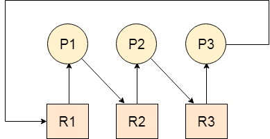
Let us assume that there are three processes P1, P2 and P3. There are three different resources R1, R2 and R3. R1 is assigned to P1, R2 is assigned to P2 and R3 is assigned to P3.

After some time, P1 demands for R1 which is being used by P2. P1 halts its execution since it can't complete without R2. P2 also demands for R3 which is being used by P3. P2 also stops its execution because it can't continue without R3. P3 also demands for R1 which is being used by P1 therefore P3 also stops its execution.

In this scenario, a cycle is being formed among the three processes. None of the process is progressing and they are all waiting. The computer becomes unresponsive since all the processes got blocked.

Difference between Starvation and Deadlock

Sr.	Deadlock	Starvation
1	Deadlock is a situation where no process got blocked and no process proceeds	Starvation is a situation where the low priority process got blocked and the high priority processes proceed.
2	Deadlock is an infinite waiting.	Starvation is a long waiting but not infinite.
3	Every Deadlock is always a starvation.	Every starvation need not be deadlock.
4	The requested resource is blocked by the other process.	The requested resource is continuously be used by the higher priority processes.
5	Deadlock happens when Mutual exclusion, hold and wait, No preemption and circular wait occurs simultaneously.	It occurs due to the uncontrolled priority and resource management.

Necessary conditions for Deadlocks

1. Mutual Exclusion

A resource can only be shared in mutually exclusive manner. It implies, if two process cannot use the same resource at the same time.

2. Hold and Wait

A process waits for some resources while holding another resource at the same time.

3. No preemption

The process which once scheduled will be executed till the completion. No other process can be scheduled by the scheduler meanwhile.

4. Circular Wait

All the processes must be waiting for the resources in a cyclic manner so that the last process is waiting for the resource which is being held by the first process.

Deadlock Characterization

A deadlock happens in operating system when two or more processes need some resource to complete their execution that is held by the other process.

A deadlock occurs if the four Coffman conditions hold true. But these conditions are not mutually exclusive. They are given as follows −

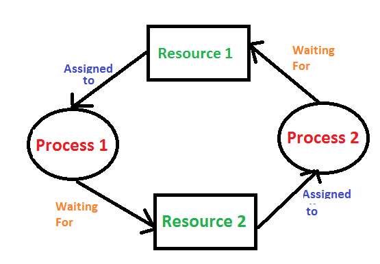
Mutual Exclusion

There should be a resource that can only be held by one process at a time. In the diagram below, there is a single instance of Resource 1 and it is held by Process 1 only.

Hold and Wait

A process can hold multiple resources and still request more resources from other processes which are holding them. In the diagram given below, Process 2 holds Resource 2 and Resource 3 and is requesting the Resource 1 which is held by Process 1.

No Preemption

A resource cannot be preempted from a process by force. A process can only release a resource voluntarily. In the diagram below, Process 2 cannot preempt Resource 1 from Process 1. It will only be released when Process 1 relinquishes it voluntarily after its execution is complete.

Circular Wait

A process is waiting for the resource held by the second process, which is waiting for the resource held by the third process and so on, till the last process is waiting for a resource held by the first process. This forms a circular chain. For example: Process 1 is allocated Resource2 and it is requesting Resource 1. Similarly, Process 2 is allocated Resource 1 and it is requesting Resource 2. This forms a circular wait loop.

Deadlock Prevention

It's important to prevent a deadlock before it can occur. The system checks every transaction before it is executed to make sure it doesn't lead the deadlock situations. Such that even a small change to occur dead that an operation which can lead to Deadlock in the future it also never allowed process to execute.

It is a set of methods for ensuring that at least one of the conditions cannot hold.

No preemptive action:

No Preemption - A resource can be released only voluntarily by the process holding it after that process has finished its task

• If a process which is holding some resources request another resource that can't be immediately allocated to it, in that situation, all resources will be released.
• Preempted resources require the list of resources for a process that is waiting.
• The process will be restarted only if it can regain its old resource and a new one that it is requesting.
• If the process is requesting some other resource, when it is available, then it was given to the requesting process.
• If it is held by another process that is waiting for another resource, we release it and give it to the requesting process.

Mutual Exclusion:

Mutual Exclusion is a full form of Mutex. It is a special type of binary semaphore which used for controlling access to the shared resource. It includes a priority inheritance mechanism to avoid extended priority inversion problems. It allows current higher priority tasks to be kept in the blocked state for the shortest time possible.

Resources shared such as read-only files never lead to deadlocks, but resources, like printers and tape drives, needs exclusive access by a single process.

Hold and Wait:

In this condition, processes must be stopped from holding single or multiple resources while simultaneously waiting for one or more others.

Circular Wait:

It imposes a total ordering of all resource types. Circular wait also requires that every process request resources in increasing order of enumeration.

Deadlock Avoidance

Deadlock Avoidance 

Deadlock avoidance can be done with Banker’s Algorithm. 

Banker’s Algorithm 

Bankers’s Algorithm is a resource allocation and deadlock avoidance algorithm which test all the request made by processes for resources, it checks for the safe state, if after granting request system remains in the safe state it allows the request and if there is no safe state it doesn’t allow the request made by the process. 

Inputs to Banker’s Algorithm:  

1. Max need of resources by each process. 
2. Currently, allocated resources by each process. 
3. Max free available resources in the system.

The request will only be granted under the below condition: 

1. If the request made by the process is less than equal to max need to that process. 
2. If the request made by the process is less than equal to the freely available resource in the system.

Example: 

Total resources in the system:

A B C D

6 5 7 6

Available system resources are:

A B C D

3 1 1 2

Processes (currently allocated resources):

    A B C D

P1  1 2 2 1

P2  1 0 3 3

P3  1 2 1 0 

Processes (maximum resources):

    A B C D

P1  3 3 2 2

P2  1 2 3 4

P3  1 3 5 0 

Need = maximum resources - currently allocated resources.

Processes (need resources):

    A B C D

P1  2 1 0 1

P2  0 2 0 1

P3  0 1 4 0

Banker's Algorithm

It is a banker algorithm used to avoid deadlock and allocate resources safely to each process in the computer system. The 'S-State' examines all possible tests or activities before deciding whether the allocation should be allowed to each process. It also helps the operating system to successfully share the resources between all the processes. The banker's algorithm is named because it checks whether a person should be sanctioned a loan amount or not to help the bank system safely simulate the allocation of resources. In this section, we will learn the Banker's Algorithm in detail. Also, we will solve problems based on the Banker's Algorithm. To understand the Banker's Algorithm first we will see a real word example of it.

Suppose the number of account holders in a particular bank is 'n', and the total money in a bank is 'T'. If an account holder applies for a loan; first, the bank subtracts the loan amount from full cash and then estimates the cash difference is greater than T to approve the loan amount. These steps are taken because if another person applies for a loan or withdraws some amount from the bank, it helps the bank manage and operate all things without any restriction in the functionality of the banking system.

Similarly, it works in an operating system. When a new process is created in a computer system, the process must provide all types of information to the operating system like upcoming processes, requests for their resources, counting them, and delays. Based on these criteria, the operating system decides which process sequence should be executed or waited so that no deadlock occurs in a system. Therefore, it is also known as a deadlock avoidance algorithm or deadlock detection in the operating system.

Advantages

The following are the essential characteristics of the Banker's algorithm:

1. It contains various resources that meet the requirements of each process.
2. Each process should provide information to the operating system for upcoming resource requests, the number of resources, and how long the resources will be held.
3. It helps the operating system manage and control process requests for each type of resource in the computer system.
4. The algorithm has a Max resource attribute that represents indicates each process can hold the maximum number of resources in a system.

Disadvantages

1. It requires a fixed number of processes, and no additional processes can be started in the system while executing the process.
2. The algorithm does no longer allows the processes to exchange its maximum needs while processing their tasks.
3. Each process has to know and state its maximum resource requirement in advance for the system.
4. The number of resource requests can be granted in a finite time, but the time limit for allocating the resources is one year.

When working with a banker's algorithm, it requests to know about three things:

1. How much each process can request for each resource in the system. It is denoted by the [MAX] request.
2. How much each process is currently holding each resource in a system. It is denoted by the [ALLOCATED] resource.
3. It represents the number of each resource currently available in the system. It is denoted by the [AVAILABLE] resource.

Following are the important data structures terms applied in the banker's algorithm as follows:

Suppose n is the number of processes, and m is the number of each type of resource used in a computer system.

1. Available: It is an array of length 'm' that defines each type of resource available in the system. When Available[j] = K, means that 'K' instances of Resources type R[j] are available in the system.
2. Max: It is a [n x m] matrix that indicates each process P[i] can store the maximum number of resources R[j] (each type) in a system.
3. Allocation: It is a matrix of m x n orders that indicates the type of resources currently allocated to each process in the system. When Allocation [i, j] = K, it means that process P[i] is currently allocated K instances of Resources type R[j] in the system.
4. Need: It is an M x N matrix sequence representing the number of remaining resources for each process. When the Need[i] [j] = k, then process P[i] may require K more instances of resources type Rj to complete the assigned work.
   Nedd[i][j] = Max[i][j] - Allocation[i][j].
5. Finish: It is the vector of the order m. It includes a Boolean value (true/false) indicating whether the process has been allocated to the requested resources, and all resources have been released after finishing its task.

The Banker's Algorithm is the combination of the safety algorithm and the resource request algorithm to control the processes and avoid deadlock in a system:

Safety Algorithm

It is a safety algorithm used to check whether or not a system is in a safe state or follows the safe sequence in a banker's algorithm:

1. There are two vectors Wok and Finish of length m and n in a safety algorithm.

Initialize: Work = Available
Finish[i] = false; for I = 0, 1, 2, 3, 4… n - 1.

2. Check the availability status for each type of resource [i], such as:

Need[i] <= Work

Finish[i] == false

If i does not exist, go to step 4.

 

3. Work = Work +Allocation(i) // to get new resource allocation

Finish[i] = true

Go to step 2 to check the status of resource availability for the next process.

 

4. If Finish[i] == true; it means that the system is safe for all processes.

Resource Request Algorithm

A resource request algorithm checks how a system will behave when a process makes each type of resource request in a system as a request matrix.

 

Let's create a resource request array R[i] for each process P[i]. If the Resource Requesti [j] is equal to 'K', which means the process P[i] requires 'k' instances of Resources type R[j] in the system.

1. When the number of requested resources of each type is less than the Need resources, go to step 2, and if the condition fails, which means that the process P[i] exceeds its maximum claim for the resource. As the expression suggests:

If Request(i) <= Need

Go to step 2;

2. And when the number of requested resources of each type is less than the available resource for each process, go to step (3). As the expression suggests:

If Request(i) <= Available

Else Process P[i] must wait for the resource since it is not available for use.

3. When the requested resource is allocated to the process by changing state:

Available = Available – Request

Allocation(i) = Allocation(i) + Request (i)

Needi = Needi - Request

When the resource allocation state is safe, its resources are allocated to the process P(i). And if the new state is unsafe, Process P (i) has to wait for each type of Request R(i) and restore the old resource-allocation state.

Example: Consider a system that contains five processes P1, P2, P3, P4, P5, and the three resource types A, B, and C. Following are the resource types: A has 10, B has 5 and the resource type C has 7 instances.

Process	Allocation A         B         C	Max A         B         C	Available A         B         C
P1	0         1          0	7         5         3	3         3         2
P2	2         0         0	3         2         2
P3	3         0         2	9         0         2
P4	2         1         1	2         2         2
P5	0         0         2	4         3         3

 

Answer the following questions using the banker's algorithm:

1. What is the reference of the need matrix?
2. Determine if the system is safe or not.
3. What will happen if the resource request (1, 0, 0) for process P1 can the system accept this request immediately?

Ans. 2: The context of the need matrix is as follows:

Need [i] = Max [i] - Allocation [i]

Need for P1: (7, 5, 3) - (0, 1, 0) = 7, 4, 3

Need for P2: (3, 2, 2) - (2, 0, 0) = 1, 2, 2

Need for P3: (9, 0, 2) - (3, 0, 2) = 6, 0, 0

Need for P4: (2, 2, 2) - (2, 1, 1) = 0, 1, 1

Need for P5: (4, 3, 3) - (0, 0, 2) = 4, 3, 1

Process	Need A         B         C
P1	7         4         3
P2	1         2         2
P3	6         0         0
P4	0         1         1
P5	4         3         1

Hence, we created the context of the need matrix.

Ans. 2: Apply the Banker's Algorithm:

Available Resources of A, B, and C are 3, 3, and 2.

Now we check if each type of resource request is available for each process.

Step 1: For Process P1:

Need <= Available

7, 4, 3 <= 3, 3, 2 condition is false.

So, we examine another process, P2.

Step 2: For Process P2:

Need <= Available

1, 2, 2 <= 3, 3, 2 conditions true

New available = available + Allocation

(3, 3, 2) + (2, 0, 0) => 5, 3, 2

Similarly, we examine another process P3.

Step 3: For Process P3:

P3 Need <= Available

6, 0, 0 < = 5, 3, 2 condition is false.

Similarly, we examine another process, P4.

Step 4: For Process P4:

P4 Need <= Available

0, 1, 1 <= 5, 3, 2 condition is true

New Available resource = Available + Allocation

5, 3, 2 + 2, 1, 1 => 7, 4, 3

Similarly, we examine another process P5.

Step 5: For Process P5:

P5 Need <= Available

4, 3, 1 <= 7, 4, 3 condition is true

New available resource = Available + Allocation

7, 4, 3 + 0, 0, 2 => 7, 4, 5

Now, we again examine each type of resource request for processes P1 and P3.

Step 6: For Process P1:

P1 Need <= Available

7, 4, 3 <= 7, 4, 5 condition is true

New Available Resource = Available + Allocation

7, 4, 5 + 0, 1, 0 => 7, 5, 5

So, we examine another process P2.

Step 7: For Process P3:

P3 Need <= Available

6, 0, 0 <= 7, 5, 5 condition is true

New Available Resource = Available + Allocation

7, 5, 5 + 3, 0, 2 => 10, 5, 7

Hence, we execute the banker's algorithm to find the safe state and the safe sequence like P2, P4, P5, P1, and P3.

Ans. 3: For granting the Request (1, 0, 0), first we have to check that Request <= Available, that is (1, 0, 0) <= (3, 3, 2), since the condition is true. So process P1 gets the request immediately.

Deadlock Detection And Recovery

Deadlock Detection

1. If resources have single instance:
   In this case for Deadlock detection we can run an algorithm to check for cycle in the Resource Allocation Graph. Presence of cycle in the graph is the sufficient condition for deadlock.
   
   

   In the above diagram, resource 1 and resource 2 have single instances. There is a cycle R1 → P1 → R2 → P2. So, Deadlock is Confirmed.

2. If there are multiple instances of resources:
   Detection of the cycle is necessary but not sufficient condition for deadlock detection, in this case, the system may or may not be in deadlock varies according to different situations.

Deadlock Recovery

A traditional operating system such as Windows doesn’t deal with deadlock recovery as it is time and space consuming process. Real-time operating systems use Deadlock recovery.

Recovery method
1. Killing the process: killing all the process involved in the deadlock. Killing process one by one. After killing each process check for deadlock again keep repeating the process till system recover from deadlock.
2. Resource Preemption: Resources are preempted from the processes involved in the deadlock, preempted resources are allocated to other processes so that there is a possibility of recovering the system from deadlock. In this case, the system goes into starvation.